Python raster stats
A common task in many of my data workflows involves summarizing geospatial raster datasets based on vector geometries (i.e. zonal statistics). Despite many alternatives (starspan, the QGIS Zonal Statistics plugin, ArcPy and R) there were none that were
- open source
- fast enough
- flexible enough
- worked with python data structures
We’d written a wrapper around starspan for madrona (see madrona.raster_stats ) but relying on shell calls and an aging, unmaintained C++ code base was not cutting it.
So I set out to create a solution using numpy, GDAL and python. The
rasterstats package was born.
`python-raster-stats` on github
Example
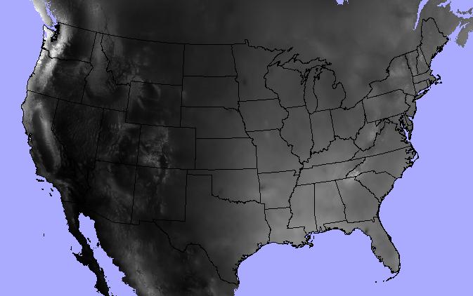
Let’s jump into an example. I’ve got a polygon shapefile of continental US state boundaries and a raster dataset of annual precipitation from the North American Environmental Atlas.

>>> states = "/data/workspace/rasterstats_blog/boundaries_contus.shp"
>>> precip = "/data/workspace/rasterstats_blog/NA_Annual_Precipitation_GRID/NA_Annual_Precipitation/data/na_anprecip/hdr.adf"
The raster_stats function is the main entry point. Provide a vector and a
raster as input and expect a list of dicts, one for each input feature.
>>> from rasterstats import raster_stats
>>> rain_stats = raster_stats(states, precip, stats="*", copy_properties=True)
>>> len(rain_stats)  # continental US; 48 states plus District of Columbia

49
Print out the stats for a given state:
>>> [x for x in rain_stats if x['NAME'] == "Oregon"][0]

{'COUNTRY': 'USA',
 'EDIT': 'NEW',
 'EDIT_DATE': '20060803',
 'NAME': 'Oregon',
 'STATEABB': 'US-OR',
 'Shape_Area': 250563567264.0,
 'Shape_Leng': 2366783.00361,
 'UIDENT': 124704,
 '__fid__': 35,
 'count': 250510,
 'majority': 263,
 'max': 3193.0,
 'mean': 779.2223903237395,
 'median': 461.0,
 'min': 205.0,
 'minority': 3193,
 'range': 2988.0,
 'std': 631.539502512283,
 'sum': 195203001.0,
 'unique': 2865}
Find the three driest states:
>>> [(x['NAME'], x['mean']) for x in
       sorted(rain_stats, key=lambda k: k['mean'])[:3]]

[('Nevada', 248.23814034118908),
 ('Utah', 317.668743027571),
 ('Arizona', 320.6157232064074)]
And write the data out to a csv.
from rasterstats import stats_to_csv
with open('out.csv', 'w') as fh:
    fh.write(stats_to_csv(rain_stats))
Geo interface
The basic usage above shows the path of an entire OGR vector layer as the first argument. But raster-stats also supports other vector features/geometries.
- Well-Known Text/Binary
- GeoJSON string and mappings
- Any python object that supports the geo_interface
- Single objects or iterables
In this example, I use a geojson-like python mapping to specify a single geometry
>>> geom = {'coordinates': [[
   [-594335.108537269, -570957.932799394],
   [-422374.54395311, -593387.5716581973],
   [-444804.1828119133, -765348.1362423564],
   [-631717.839968608, -735441.9510972851],
   [-594335.108537269, -570957.932799394]]],
 'type': 'Polygon'}

>>> raster_stats(geom, precip, stats="min median max")

[{'__fid__': 0, 'max': 1011.0, 'median': 451.0, 'min': 229.0}]
Categorical
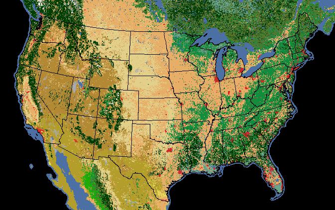
We’re not limited to descriptive statistics for continuous rasters either; we can get unique pixel counts for categorical rasters as well. In this example, we’ve got a raster of 2005 land cover (i.e. general vegetation type).

Note that
we can specify only the stats that make sense and the categorical=True
provides a count of each pixel value.
>>> landcover = "/data/workspace/rasterstats_blog/NA_LandCover_2005.img"
>>> veg_stats = raster_stats(states, landcover,
    stats="count majority minority unique",
    copy_properties=True,
    nodata_value=0,
    categorical=True)
>>> [x for x in veg_stats if x['NAME'] == "Oregon"][0]

{1: 999956,
 3: 6,
 5: 3005,
 6: 198535,
 8: 2270805,
 10: 126199,
 14: 20883,
 15: 301884,
 16: 17452,
 17: 39246,
 18: 28872,
 19: 2174,
 'COUNTRY': 'USA',
 'EDIT': 'NEW',
 'EDIT_DATE': '20060803',
 'NAME': 'Oregon',
 'STATEABB': 'US-OR',
 'Shape_Area': 250563567264.0,
 'Shape_Leng': 2366783.00361,
 'UIDENT': 124704,
 '__fid__': 35,
 'count': 4009017,
 'majority': 8,
 'minority': 3,
 'unique': 12}
Of course the pixel values alone don’t make much sense. We need to interpret the pixel values as land cover classes:
Value, Class_name
1       Temperate or sub-polar needleleaf forest
2       Sub-polar taiga needleleaf forest
3       Tropical or sub-tropical broadleaf evergreen
4       Tropical or sub-tropical broadleaf deciduous
5       Temperate or sub-polar broadleaf deciduous
6        Mixed Forest
7       Tropical or sub-tropical shrubland
8       Temperate or sub-polar shrubland
9       Tropical or sub-tropical grassland
10      Temperate or sub-polar grassland
11      Sub-polar or polar shrubland-lichen-moss
12      Sub-polar or polar grassland-lichen-moss
13      Sub-polar or polar barren-lichen-moss
14      Wetland
15      Cropland
16      Barren Lands
17      Urban and Built-up
18      Water
19      Snow and Ice
So, for our Oregon example above we can see that, despite Oregon’s reputation as a lush green landscape, the majority land cover class (#8) is “Temperate or sub- polar shrubland” at 2.27m pixels out of 4 millions total.
There’s a lot more functionality that isn’t covered in this post but you get the picture… please check it out and let me know what you think.
blog comments powered by Disqus
