For all the benefits of KML, it is decidedly a step backwards for handling large vector datasets. Most KML clients, including the cannonical Google Earth application, experience debilitating slow-down when viewing a couple dozen MB of vector data - datasets that I could easily open on a Pentium 4 in ArcView 3.2 10 years ago!

The unfortunate reality is that optimizing the performance of KML datasets is conflated with the structure of the data and is thus the responsibility of the data publisher. The wisdom of combining styling, performance-related structure, organizational structure, geometry and attributes into a single file format may be questionable, but KML has become the defacto geographic markup language due to it’s other benefits.

Anyways, back to performance enhancements on big vector datasets… The concept of “regionation” is used by several KML software to improve performance. From the Google LatLong Blog:

You can think of Regionation as a hierarchical subdivision of points or tiles, which shows less detail from afar, and more detail as you zoom in to the globe. This dynamic loading creates clearer visualizations by minimizing clutter, while simultaneously speeding up the rendering process.

In most implementations, there is a generic strategy for determining this hierarchy based on attributes or geometry size (in the case of vectors) or by a tile system. Neither is ideal when you want to preserve the vector nature of the data, split it into small, easily-loadable files and determine it’s view based on the natural hierarchy that is built into the data structure.

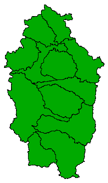
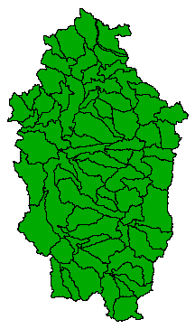
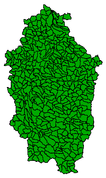
Specifically I am thinking about watersheds here - the US Hydrologic Units. Hydrologic units are watershed boundaries that are organized in a nested hierarchy; higher levels contain smaller watersheds that are contained within a single watershed from a “parent” level. The unique identifiers (hydrologic unit codes or HUCs) are rather ingenious as well; Each level is represented by 2 digits and are concatenated to form a single identifier that can be used to determine it’s “parent”. For example:

Level 4 HUCs
e.g. 17090011

Level 5 HUCs
e.g. 1709001104

Level 6 HUCs
e.g. 170900110403

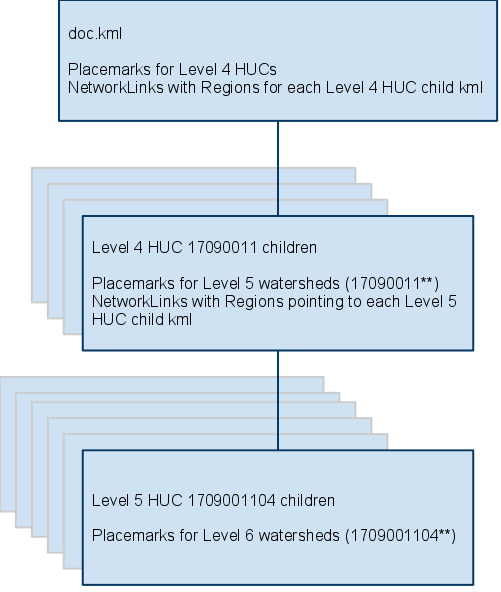
Instead of fabricating a hierarchy of features, why not just use this natural hierarchy to structure the KML documents?

Or as KML markup:

    <placemark>
        <name>17090009</name>
        <styleurl>#HUC_8-default</styleurl>
        <polygon><outerboundaryis><linearring><coordinates>...
        </coordinates></linearring></outerboundaryis></polygon>   
    </placemark>
    
    <networklink>
    <name>17090009_children</name>
    <region>
      <latlonaltbox>
        <west>-123.001645628</west>
        <south>44.8300083641</south>
        <east>-122.203351254</east>
        <north>45.298653051</north>
      </latlonaltbox>
      <lod>
        <minlodpixels>256</minlodpixels>
        <maxlodpixels>1600</maxlodpixels>
      </lod>
    </region>
    <link>
      <href>./17090009_children.kml</href>
      <viewrefreshmode>onRegion</viewrefreshmode>
    </link>
    </networklink>

The advantages to this design are that you don’t have to break the geometries up to fit into a square tiling pattern, data loads and renders in a logical pattern and there will always be 100 or less (usually far less) placemarks per file due to the design of the HUC data structure. File sizes stay low, network links load quickly and request/rendering occurs only when they come into view. For this example dataset totaling 300M of shapefiles, there are several hundred resulting kmz files without any repeated features and all less than ~ 150K each. In essence, it achieves optimal performance by its very design.

Here’s a video of it in action:

This was all done with a fairly “hackish” python script. I’ll continue to refine it as needed for this particular application but, at this time, it’s not intended to be a reusable tool - if you want to use it, be prepared to dig through the source code and get your hands dirty. The same concept could theoretically be applied to any spatially-hierarchical vector data (think geographic boundaries … country > state > county > city).